This simple 3D example consists in reading an initial mesh of a cube, adapting it using a smaller
specified edge size, and writing the final adapted mesh.
import pyamg, math, numpy as np
def analytical_fun(x,y,z=1):
xyz = (x-0.4)*(y-0.4)*(z-0.4)
if( xyz <= (-1.*math.pi/50.)): return 0.1*math.sin(50.*xyz)
elif(xyz <= 2.*math.pi/50.): return math.sin(50.*xyz)
else: return 0.1*math.sin(50.*xyz)
def create_sensor(mesh):
sensor = []
crd = []
if ( 'xyz' in mesh ):
crd = mesh['xyz']
for x in crd:
sensor.append(analytical_fun(x[0],x[1],x[2]))
elif ( 'xy' in mesh ):
crd = mesh['xy']
for x in crd:
sensor.append(analytical_fun(x[0],x[1]))
return sensor
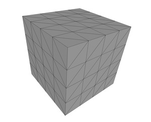
# Load mesh
msh3d = pyamg.read_mesh("cube.meshb")
# Create the sensor for adaptation
msh3d['sensor'] = create_sensor(msh3d)
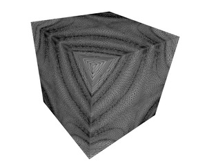
Then, the 'Lp' remeshing option is set such that the
interpolation error of the sensor will be controled in L^2 norm. Five adaptive iterations are
performed to capture the anisotropy, and the final mesh is outputted.
Mesh adaptation according to an isotropic sizing field
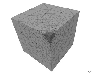
Here, an isotropic refinement using a sizing field is shown. This is done using the key "Metric" in the mesh data
structure. We illustrate this through the refinement around the corner (0,0,0) of the unit cube.
This example uses the geometry and the flow conditions of the Inviscid ONERA M6 SU2 test case.
Freestream Pressure = 101325.0 N/m2
Freestream Temperature = 273.15 K
Freestream Mach number = 0.8
Angle of attack (AoA) = 1.25 deg
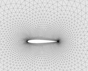
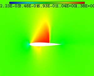
The goal of this mesh adaptation is to accurately capture the shocks around the airfoil, by creating
anisotropic mesh elements along the shocks' directions of anisotropy. The Mach number is used as the
sensor for mesh adaptation.
SU2 configuration file options
% ------------- MESH ADAPTATION PARAMETER ------------%

% Mesh size parameters
ADAP_SIZES= (100, 200, 300)

% Number of iterative loops performed for each mesh size
ADAP_SUBITE= (2, 2, 2)

% Number of CFD iterations for each mesh size
ADAP_EXT_ITER= (500, 500, 500)

% Prescribed residual reduction for each mesh size
ADAP_RESIDUAL_REDUCTION= (3, 3, 3)

% Sensor used for mesh adaptation
% (MACH, PRES, or MACH_PRES)
ADAP_SENSOR=  MACH

% Max and min edge sizes
ADAP_HMAX=  200
ADAP_HMIN=  1e-8

% Prescribed mesh gradation
ADAP_HGRAD= 1.3

% Output adapted mesh
MESH_OUT_FILENAME= mesh_NACA0012_adap.su2

% Final adapted restart solution
RESTART_FLOW_FILENAME= NACA0012_adap.dat

% Initial restart solution
SOLUTION_FLOW_FILENAME= NACA0012_ini.dat
Running the case
The mesh adaptation process is started by running the following command line in a terminal:
where the -n option corresponds to the desired number of
processing cores.
A ./ADAP folder is created, in which the successive calls to
SU2_CFD and pyAMG are performed. Once all the adaptive iterations are done, the final adapted mesh
and restart solution are outputted in the current directory.
Results
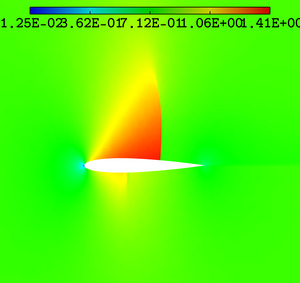
A comparison of the initial and final meshes/solutions is shown in the figures below.
NACA0012: initial surface mesh and solution (5233 vertices).NACA0012: adapted surface mesh and solution (21100 vertices).
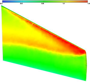
This example uses the geometry and the flow conditions of the Inviscid ONERA M6 SU2 test case.
Freestream Pressure = 101325.0 N/m2
Freestream Temperature = 288.15 K
Freestream Mach number = 0.8395
Angle of attack (AoA) = 3.06 deg
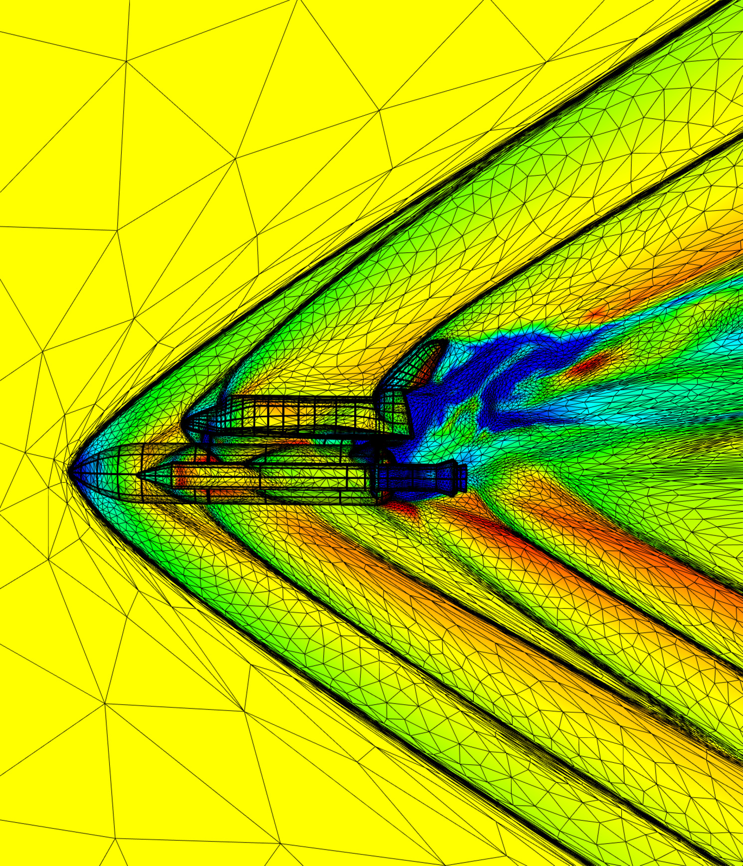
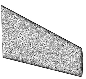
The goal of this mesh adaptation is to accurately capture the typical "lambda" shock along the upper
surface of the lifting wing, by creating anisotropic mesh elements along the shock's directions of
anisotropy. The Mach number is used as the sensor for mesh adaptation.
SU2 configuration file options
% -- MESH ADAPTATION PARAMETER --%

% Mesh size parameters
ADAP_SIZES= (2000, 4000, 8000)

% Number of iterative loops performed for each mesh size
ADAP_SUBITE= (2, 2, 2)

% Number of CFD iterations for each mesh size
ADAP_EXT_ITER= (1000, 1000, 1000)

% Prescribed residual reduction for each mesh size
ADAP_RESIDUAL_REDUCTION= (3, 3, 3)

% Sensor used for mesh adaptation
% (MACH, PRES, or MACH_PRES)
ADAP_SENSOR=  MACH

% Max and min edge sizes
ADAP_HMAX=  200
ADAP_HMIN=  1e-8

% Prescribed mesh gradation
ADAP_HGRAD= 1.3

% Output adapted mesh
MESH_OUT_FILENAME= M6_adap.su2

% Final adapted restart solution
RESTART_FLOW_FILENAME= M6_adap.dat
Running the case
The mesh adaptation process is started by running the following command line in a terminal:
$ mesh_adaptation_amg.py -f adap_ONERAM6.cfg -n 4
where the -n option corresponds to the desired number of
processing cores.
A ./ADAP folder is created, in which the successive calls to
SU2_CFD and pyAMG are performed. Once all the adaptive iterations are done, the final adapted mesh
and restart solution are outputted in the current directory.
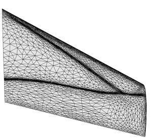
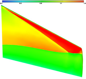
Results
A comparison of the initial and final meshes/solutions is shown in the figure below. The lambda
shock resolution is improved, while reducing the number of mesh vertices.
ONERA M6 wing: initial surface mesh and solution (141537 vertices).ONERA M6 wing: adapted surface mesh and solution (48299 vertices).